Adaptation of Mathematical ALGorithms

Ford-Fulkerson algorithm is used to find the maximum flow in a flow network. We work with a network , where  is a set of nodes including a source  and sink  is a set of directed edges. A label of an edge is written as where  indicates its capacity and  means a flow (amount of energy) streaming through the edge.

1. At the beginning of the algorithm set the flow of all the edges to .
2. We repeatedly search for the augmenting path from the source  to the sink . As soon as we find such a path we also compute the available capacity of all its edges, by which we subsequently increase the flow in the network.

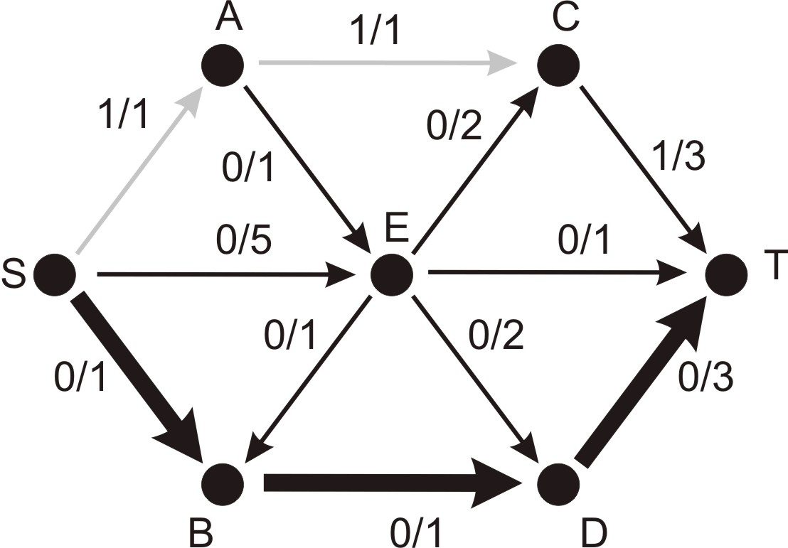
When processing the algorithm in the standard way we work with a visual representation of the network and modify labels of edges. Image 1 illustrates a network  with seven nodes and the current flow (see the path ). The augmenting path , with the available capacity on all its edges is highlighted. In the next step we can increase the flow and modify labels of the augmenting path, change to for the paths , and to for the path .

Example 1: network 

Image 1: Network  with the flow where the augmenting path is highlighted

To demonstrate Ford-Fulkerson algorithm we come with an Animation 1 of the computation and use a concrete flow network.

1. Work with a network on a sheet of a spreadsheet editor:

The network is again converted to a table and organized in a similar way as in the case of the first method of Dijsktra's algorithm adaption. We add labels of the nodes to the first column. All the other cells on the row for a node  are reserved for the edges coming out from  and are written as – where  is the end node of the edge,  indicates the current flow through the edge and  identifies its capacity. Let us take the same network  illustrated on the Image 1. The following Table 1 demonstrates the situation after processing the first augmenting path

Example 3: network 

	–	–	–
	–	–
	–
	–
	–
	–	–	–	–

Tabulka 1: Network  converted to a table after processing the first augmenting path

A blind student finds an augmenting path from the source  to the sink . He/she consecutively goes through the table and holds a sequence of the path's nodes and actual available capacity of the path's edges in his/her memory. During the second view he/she modifies the flow and marks edges with the flow equal to the capacity, which are directed from the source to the sink.

2. Edges are organized one below each other on lines of a standard text editor:

every edge is written separately on one line as ––, where  is a starting node and  is an ending node of the edge with a capacity  and a current flow . The edges are ordered alphabetically according to the node from which they come. We work in a similar way as when using the previous method. We go through the table twice, first to find an augmenting path from the source to the sink, then to increase a flow on the path.

The first method was evaluated as the better one. It is easy to find the desired information in the table and to search for an augmenting path (Let us mention that it is difficult to find a maximum flow if we need to search for the augmenting path containing edges in the opposite direction.). When going through the graph using the second method a blind student has to observe many lines with data not relevant at the moment. We recommend students to make a note about the processed augmenting path in a temporary text file (it suffices to write down a sequence of nodes from the source to the sink).